")
Trees are a popular supervised learning algorithm with benefits including their ability to be used for regression and classification and ease of interpretation. However, decision trees are not the most performing algorithm, and because the training data differs little, it is easy to overfit. This can lead to completely different trees. This is why people often turn to ensemble models like bag trees and random forests. These are trained in multiple decision trees that are trained in bootstrap data and aggregated to achieve better predictive performance than any tree can provide. This tutorial includes the following:
- What is packaging
- What makes random forests unique
- Training and tuning random forests with Scikit-Learn
- Calculate and interpret the importance of features
- Visualizing a single decision tree in a random forest
As always, the code used in this tutorial is available on my github. My YouTube channel is also available in the video version of this tutorial for those who like to follow visually. So, let’s get started!
What is packaging (Bootstrap aggregation)
Random forests can be classified as packaging algorithms (bOOTSTRAP aggregat). The bag consists of two steps:
1.) Boot sampling: Create multiple training sets, draw samples randomly, and replace them from the original dataset. These new training sets (called bootstrap datasets) usually contain the same number of rows as the original dataset, but a single row may appear multiple times or not at all. On average, each bootstrap dataset contains 63.2% of the unique rows from the original data. The remaining ~36.8% of rows are excluded and can be used for out-of-bag (OOB) evaluation. For more information on this concept, see my Sampling with or without alternative blog posts.
2.) Summary prediction: Each bootstrap dataset is used to train different decision tree models. The final prediction is made by combining the outputs of all single trees. For classification, this is usually done by majority vote. For regression, the predictions are average.
Training each tree on different bootstrap samples introduces changes across trees. Although this does not completely eliminate correlation, especially when certain functions dominate, it helps to reduce overfitting combined with aggregation. Average predictions for many such trees reduce overall variance Ensemble, improve summary.
What makes random forests unique

Assume that there is a powerful feature in your dataset. In bagged trees, each tree may be repeatedly divided on this feature, resulting in the relevant tree, while aggregation benefits less. Random forests reduce this problem by introducing further randomness. Specifically, they changed the way they chose to split during training:
1). Create an N boot dataset. Note that while bootstrapping is usually used for random forests, it is not strictly necessary, as step 2 (random feature selection) introduces enough diversity among trees.
2). For each tree, on each node, a random subset of features is selected as candidates, from which the best split is selected. In Scikit-Learn, this is max_features Parameters, default 'sqrt' for classifiers and 1 Used for regressors (equivalent to wrapped trees).
3). Summary forecast: Voting for classification and mean regression.
Note: Random forests use substitutions to guide sampling and sampling of the dataset without substitutions to select a subset of features.

Out of Band (OOB) Score
Because ~36.8% of the training data is excluded from any given tree, you can use this retention section to evaluate the predictions of that tree. Scikit-learn allows this permission by the OOB_SCORE = TRUE parameter, thus providing an efficient way to estimate generalization errors. You will see this parameter in the training example, later in the training example.
Training and tuning Scikit-Learn’s random forest
Because of their simplicity, interpretability, and ability, random forests remain a strong baseline for tabular data, as each tree is independently trained. This section demonstrates how to load data, perform train test splits, train baseline models, adjust hyperparameters using grid search, and evaluate the final model in the test set.
Step 1: Training the baseline model
Before tuning, it is best to train the baseline model with reasonable default values. This gives you an initial sense of performance and can be verified using an out-of-bag (OOB) score built into packaging-based models such as Random Forest. This example uses the King County dataset’s Home Sales (CCO 1.0 General License), which includes real estate sales in the Seattle area between May 2014 and May 2015. This approach allows us to preserve the test set after adjustments for the final evaluation.
Python"># Import libraries

# Some imports are only used later in the tutorial
import matplotlib.pyplot as plt

import numpy as np

import pandas as pd

# Dataset: Breast Cancer Wisconsin (Diagnostic)
# Source: UCI Machine Learning Repository
# License: CC BY 4.0
from sklearn.datasets import load_breast_cancer

from sklearn.ensemble import RandomForestClassifier

from sklearn.ensemble import RandomForestRegressor

from sklearn.inspection import permutation_importance

from sklearn.model_selection import GridSearchCV, train_test_split

from sklearn import tree

# Load dataset
# Dataset: House Sales in King County (May 2014–May 2015)
# License CC0 1.0 Universal
url = '

df = pd.read_csv(url)

columns = ['bedrooms',

            'bathrooms',

            'sqft_living',

            'sqft_lot',

             'floors',

             'waterfront',

             'view',

             'condition',

             'grade',

             'sqft_above',

             'sqft_basement',

             'yr_built',

             'yr_renovated',

             'lat',

             'long',

             'sqft_living15',

             'sqft_lot15',

             'price']

df = df[columns]

# Define features and target

X = df.drop(columns='price')

y = df['price']

# Train/test split

X_train, X_test, y_train, y_test = train_test_split(X, y, random_state=0)

# Train baseline Random Forest

reg = RandomForestRegressor(

    n_estimators=100,        # number of trees

    max_features=1/3,        # fraction of features considered at each split

    oob_score=True,          # enables out-of-bag evaluation

    random_state=0

)

reg.fit(X_train, y_train)

# Evaluate baseline performance using OOB score

print(f"Baseline OOB score: {reg.oob_score_:.3f}")
Step 2: Adjust hyperparameters through grid search
While the baseline model gives a strong starting point, performance can often be improved by tuning key hyperparameters. Grid search cross-validation, by GridSearchCVsystematically explore the combination of hyperparameters and use cross-validation to evaluate each, thus selecting the configuration with the highest validation performance. The most common tuning hyperparameters include:
n_estimators: Number of decision trees in the forest. More trees can improve accuracy, but will increase training time.max_features: The number of features to consider when looking for the best split. Lower values reduce the correlation between trees.max_depth: The maximum depth of each tree. Lighter trees are faster, but may not be enough.min_samples_split: The minimum number of samples required to split the internal node. Higher values can reduce overfitting.min_samples_leaf: The minimum number of samples required at the leaf node. Helps control tree size.bootstrap: Whether to use boot samples when building trees. If it is wrong, use the entire dataset.
param_grid = {

    'n_estimators': [100],

    'max_features': ['sqrt', 'log2', None],

    'max_depth': [None, 5, 10, 20],

    'min_samples_split': [2, 5],

    'min_samples_leaf': [1, 2]

}

# Initialize model

rf = RandomForestRegressor(random_state=0, oob_score=True)

grid_search = GridSearchCV(

    estimator=rf,

    param_grid=param_grid,

    cv=5,             # 5-fold cross-validation

    scoring='r2',     # evaluation metric

    n_jobs=-1         # use all available CPU cores

)

grid_search.fit(X_train, y_train)

print(f"Best parameters: {grid_search.best_params_}")

print(f"Best R^2 score: {grid_search.best_score_:.3f}")
Step 3: Evaluate the final model of the test set
Now that we have selected the best performance model based on cross-validation, we can evaluate it in a fixed test set to estimate its generalized performance.
# Evaluate final model on test set

best_model = grid_search.best_estimator_

print(f"Test R^2 score (final model): {best_model.score(X_test, y_test):.3f}")
The importance of calculating the characteristics of random forests
One of the key advantages of random forests is their interpretability – large language models (LLMSs) are often lacking. Despite their powerful capabilities, LLMs often act as black boxes and may exhibit unrecognizable bias. In contrast, Scikit-Learn supports two main methods for measuring the importance of traits in random forests: mean reductions in impurities and permutations.
1). Average reduction in impurities (MDI): Also known as the importance of Gini, this method calculates the overall reduction in impurities brought by each feature in all trees. It’s quick and through reg.feature_importances_. However, the importance of impurity-based features can be misleading, especially for features with high cardinality (many unique values), as these functions are more likely to be simply because they provide more potential points.
importances = reg.feature_importances_

feature_names = X.columns

sorted_idx = np.argsort(importances)[::-1]

for i in sorted_idx:

    print(f"{feature_names[i]}: {importances[i]:.3f}")
2). Permutation Importance: This method evaluates the decline in model performance when the values of a single feature are randomly shuffled. Unlike MDI, it illustrates feature interaction and correlation. It’s more reliable, but it’s more computationally expensive.
# Perform permutation importance on the test set

perm_importance = permutation_importance(reg, X_test, y_test, n_repeats=10, random_state=0)

sorted_idx = perm_importance.importances_mean.argsort()[::-1]

for i in sorted_idx:

    print(f"{X.columns[i]}: {perm_importance.importances_mean[i]:.3f}")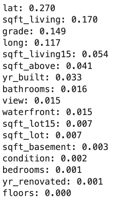
It is important to note that our geographical features LAT and Long can also be used for visualization, as shown in the figure below. Companies like Zillow are likely to make extensive use of location information in their valuation models.

Visualizing a single decision tree in a random forest
A random forest consists of multiple decision trees – each estimator passes n_estimators scope. After training the model, you can access these individual trees through the .Estimators_ attribute. Visualizing some of these trees can help illustrate the different extent of data caused by each tree for each split sample and each separate random feature selection. While earlier examples used RandomForestRegressor, here we demonstrate this visualization using RandomForestClassifier (CC by 4.0 license) trained on the Wisconsin breast cancer dataset to highlight the versatility of random forests in regression and classification tasks. This short video demonstrates what the 100 trained estimators in this dataset look like.
Fit for random forest models using Scikit-Learn
# Load the Breast Cancer (Diagnostic) Dataset

data = load_breast_cancer()

df = pd.DataFrame(data.data, columns=data.feature_names)

df['target'] = data.target

# Arrange Data into Features Matrix and Target Vector

X = df.loc[:, df.columns != 'target']

y = df.loc[:, 'target'].values

# Split the data into training and testing sets

X_train, X_test, Y_train, Y_test = train_test_split(X, y, random_state=0)

# Random Forests in `scikit-learn` (with N = 100)

rf = RandomForestClassifier(n_estimators=100,

                            random_state=0)

rf.fit(X_train, Y_train)
Plot a single estimator from a random forest using matplotlib (decision tree)
You can now view all single trees from the fitted model.
rf.estimators_

Now you can visualize a single tree. The following code visualizes the first decision tree.
fn=data.feature_names

cn=data.target_names

fig, axes = plt.subplots(nrows = 1,ncols = 1,figsize = (4,4), dpi=800)

tree.plot_tree(rf.estimators_[0],

               feature_names = fn,

               class_names=cn,

               filled = True);

fig.savefig('rf_individualtree.png')
While drawing many trees may be difficult to explain, you may want to explore the diversity across estimators. The following example shows how to visualize the first five decision trees in a forest:
# This may not the best way to view each estimator as it is small

fig, axes = plt.subplots(nrows=1, ncols=5, figsize=(10, 2), dpi=3000)

for index in range(5):

    tree.plot_tree(rf.estimators_[index],

                   feature_names=fn,

                   class_names=cn,

                   filled=True,

                   ax=axes[index])

    axes[index].set_title(f'Estimator: {index}', fontsize=11)

fig.savefig('rf_5trees.png')
in conclusion
Random forests consist of multiple decision trees trained on bootstrap data to achieve better predictive performance than obtained from any individual decision tree. If you have questions or ideas about this tutorial, feel free to go through YouTube or x.


